Serial Data Communications

We all know that the world is going to IP for almost all communications.  Despite this trend, it is a fact of life that a great deal of industrial communications still employ serial protocols such as RS232, RS422 and various flavours of RS485.

This is partly because of inertia due to the fact that a huge installed base of systems has mostly been working without problems for many years and partly because setting up a serial data comms link is usually pretty straightforward and doesn’t require advanced network design skills.  While all this is mostly true it is also true that it helps to know what you are doing.  And the first step to this is understanding the various standards that are used for most serial data links.

One of the most popular serial standards is RS232.  This is a long established standard used for relatively low-speed serial data communications used only in single point to point transmission, for example, between your Personal Computer and its serial devices.  RS232 typically is used to transmit data at up to 19.2kbps (occasionally higher) over distances of tens of meters.  It is a single ended system meaning that it transmits the signal over one wire plus a ground return path as shown in Figure 1 below.
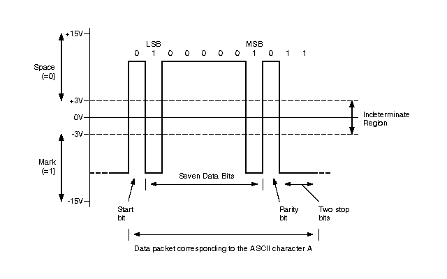
Fig1

Figure 1

In the idle state, i.e. when no data is being transmitted, the driver output will be between -5V to -15V and change to +5V to +15V when a logical “0” is being transmitted.  While the standard does not specify the state of the receiver’s output when its input is in the range -3V to +3V real RS232 line receivers generally have a threshold voltage of about +1.5V.

RS232 has three basic limitations:

  • Electrical interference can be easily induced into the signal by external noise sources
  • Interference (or crosstalk) between signals in the same cable rapidly increases with increasing cable length and/or data speeds to the point where the signal is unreadable
  • Achievable distances are not great: typically 20 to 50 meters for data rates up to 19.2kbps with fairly ordinary cable and perhaps twice this with low capacitance cable.

As an example of really poor practice, OSD once had a customer using a single twisted pair to carry transmit and receive data at about 9.6kbps.  The crosstalk made this unworkable after just a few meters!

Enter the world of RS422 and RS485. These two standards differ from RS232 in that they use differential data transmission which allows higher data rates over longer distances and with much greater noise immunity.

What exactly is differential data transmission?
RS232 uses only a single signal wire where a voltage level on that one wire is used to transmit/receive binary 1 and 0 as shown in Figure 1 above. On the other hand, differential transmission utilizes a pair of wires where a voltage difference is used to transmit/receive binary information.  This means that electrical interference will affect both wires equally so that the differential signal is still clean provided the two wires are closely coupled.  Which is why such systems use twisted pairs.

Fig2

Figure 2  RS422 Point  to Point Transmission


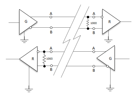
RS422 is primarily designed for point to point transmission, with one pair of wires for one direction and another pair for the other direction as shown in Figure 2 above.   Normally the twisted pairs are terminated with a termination resistor equal to the characteristic impedance of the line, typically about 100 to 150Ω.  It is possible to have multiple RS422 receivers connected (up to 10 using EIA standard receivers but more than 200 with many proprietary receivers) to the one driver but only one termination resistor is permissible.

Owing both to the intrinsic immunity to noise and crosstalk, and to the fact that twisted pairs have a well controlled characteristic impedance, transmission distances of RS422 are far greater than RS232: up to hundreds of meters at speeds as high as 10Mbps with high quality cable.

While RS422 is defined by the EIA Standard as usable in multi-drop applications it cannot be used to construct a truly multi-point network in which multiple transmitters and receivers exist in a “bus” configuration where any node can transmit or receive data.  For this we need RS485.

The RS485 standard allows up to 32 drivers and 32 receivers in a multi-point network configuration using just one or two twisted pairs as shown in Figure 3 below.

Fig3

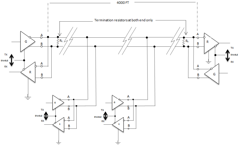
Figure 3  RS485 Two Wire Multidrop Network

2-wire RS485 allows for either Master-Slave or Peer-Peer operation with the limitation that data is transmitted in half duplex mode which means that only one device in the network can transmit at any one time.

4-wire RS485 is normally used in Master-Slave networks in which one twisted pair transmits data only from the Master to all Slaves and the other twisted pair carries return data from the Slaves to the Master as shown in Figure 4 below.

2-wire 485 networks have the advantage of lower wiring costs whilst still allowing for nodes to communicate amongst themselves.  On the downside, two-wire mode is limited to half-duplex and requires attention to turn-around delay.  4-wire networks allow full-duplex operation, but are limited to Master-Slave situations.

Fig4

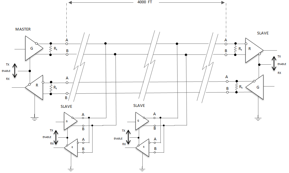
Figure 4 RS485 Four Wire Multidrop Network

One issue with both RS422 and RS485 is the need for a connection between the signal grounds of all devices in the network.  This ground connection would not be necessary if the RS422 or RS485 receivers were perfect receivers of differential signals since they would be unaffected by the common mode voltage on the differential signal.  Unfortunately, real receivers are not perfect and can usually only tolerate common mode voltages of about -7V to +12V.  If the signal grounds are not connected it is possible for a common mode voltage of tens of volts peak to peak (typically induced 50 or 60Hz AC mains hum) to be riding on the differential signal.  Sometimes such signals are enough to cause damage but more typically they just cause corruption of the data.  It is common within the surveillance market to see no ground connection between RS485 type equipment.  Such systems are basically relying on equipment safety grounds maintaining common mode voltages within the -7V to +12V range.  They usually work but you should not rely on them unless techniques such as optical isolation are used.  Some systems are actually galvanically isolated from each other and it is possible then to make a psuedo ground connection but such systems are few and far between.

A very major difference between RS422 and RS485 is due to the way RS485 drivers connect to the cable.  RS422 drivers are always turned on, ie they are either logic High or logic Low and have an output impedance of 10 to 40 ohms in either state so it is not possible to have two such drivers connected to the same twisted pair: they’d just load each other down too much.  So for multiple drivers on the one pair it is necessary that only one unit at a time is activated and the others are in a high impedance state (“tristated”) so they don’t load down the line.  There are a number of ways of controlling this state which will not be covered here but a key consequence is that during periods of inactivity the line will be in a undetermined state. How do the RS485 transceivers in a network know when to receive and when to transmit?

The most common solution is that all units default to the “Listening” state in which their drivers are tristated: as soon as activity is detected on the line the unit receives the signal and its logic ensures that it cannot transmit while receiving.  There is a turnaround time associated with this which is why many RS485 modems have an adjustable time which is typically about 10 X the bit period.  For example, if a link is running at 9600 baud, the bit time is about 105uS so the time would be set to a minimum of 1mS.  These times are usually not critical.

Biassing an RS485 Network

Connecting an RS485 network can have its issues. The EIA RS485 Specification labels the data wires “A” and “B”, although some manufacturers label these wires “+” and “-“.  A reason as to why many systems have trouble transmitting and receiving data is due to this ambiguity.  It is important to note that regardless of the polarity, it must be kept consistent throughout the whole network.

One issue with this is that when the bus is inactive it is important that it’s A and B wires be in a known state so that the first bit of a transmission is detected.  This is why biasing resistors are used to pull the two wires into the inactive state with wire A pulled towards Ground and B is pulled towards +3.3V.  As an example, in a 2-wire network of several nodes there will often be a 120Ω termination resistor at each end so to keep a reverse bias of 200mV there must be at least 3.5mA flowing through the 60Ω (two 120Ω in parallel) equivalent load.  This means that with a 3.3V system the resistors must each be about 450Ω.  This is shown in Figure 5 below.

fig5

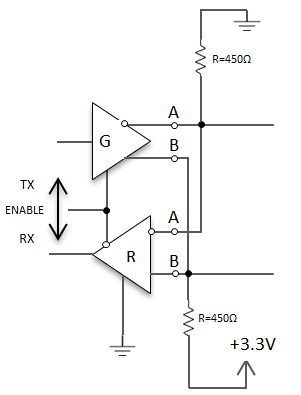
Figure 5  Use of bias Resistors in a 2 Wire RS485 Network

In such systems it is essential that the same wires (A or B) are connected throughout the network as otherwise there can be a locked out condition which kills all transmission.  Such a situation is often indicated by the modem indicators at each end of the link showing permanent a transmit state at one end with the other end showing a permanent receive state.

We have now very quickly covered the basics of RS422 and RS485.  In the next Tech note we will discuss common problems out in the real world with these standards.

Testing the Capabilities of your Ethernet Network – Part II

Before we go in to details of tests that should be performed on a L2 switch, let us look at its internal workings. Figure 1 below shows the data paths inside a multiport Gigabit layer 2 switch with major functional blocks that process the frames as they traverse the device.

Fig 1: Switch Data Flow Diagram

Fig 1: Switch Data Flow Diagram

PHY – Physical interface to receive and transmit frame to and from a port’s Gigabit MAC.

GMAC – Gigabit Media Access Controller responsible for frame formatting, frame stripping, FCS (Frame Check Sequence), CSMA/CD handling and collision handling.

Ingress Policy – Used to modify the normal flow of frames through the switch. Ingress policies examine an incoming frame for Quality of Service (QoS) priority information for the Queue Controller. These ingress policies determine the states of the switch management ports and implement features like Port Based VLANs or 802.1Q VLANs (tag processing).

Queue Controller – The brain of the switch which controls the switching architecture.

Output Queues – The output queues transmit the received packets in the order received for any given priority. These queues empty at different rates depending on port speeds or network congestion.

Egress Policy – Egress policy examines outgoing frames and modifies them (Tagging/Un-tagging frames based on 802.1Q or Port based VLANs) as they exit the switch.

Now that we have briefly described the main logic blocks of a switch, let’s discuss some of the testing scenarios.

RFC 2889 Tests

The following tests are as per RFC 2889 for different port traffic patterns, traffic loads and frame sizes.

Forwarding Rate, Throughput and Frame Loss

RFC2889 is thorough in its approach to testing layer 2 switches. It takes in to account different traffic scenarios such a fully meshed traffic pattern, partially meshed and non-meshed pattern to test forwarding rate (max frames per second), throughput (maximum load with no frame loss), frame loss and flood count which is the number of frames output from a switch port that are not specifically addressed (destination MAC) to a device connected to that port.

A brief description of the traffic patterns in as follows,

Fully Meshed: Many to ManyThis test determines if the L2 switch can handle a full mesh of traffic (from all-ports to all-ports) at various traffic loads (Fig 1). Fully meshed traffic stresses the switch fabric, fully exercises the forwarding tables and reveals weaknesses in resource allocation mechanisms.

Fig 2. Fully Meshed Traffic Pattern

Fig 2. Fully Meshed Traffic Pattern

Partially Meshed: One to Many/Many to oneTraffic is sent from one to many ports or many to one port in this pattern. This type of port traffic pattern stresses the three main logic sections of a switch: the ingress data path interface; the switch fabric that connects the ingress ports to egress ports; and, the egress data path interface. Caution should be used in the many-to-one test to avoid oversubscribing the “one” port.

Fig 3. Partially Meshed Traffic: One to Many/Many to one.

Fig 3. Partially Meshed Traffic: One to Many/Many to one.

Partially Meshed: Multiple DevicesIn this traffic pattern two L2 switches are connected to each other by one high speed backbone link. Forwarding rates can be affected by the serialization time or packet transmission time per switch hop if the packets are stored several times between source and destination. If there are more than two devices connected in a bus configuration, serialization delay is incurred for every hop along the path.

Fig 4. Partially Meshed Multiple Device Configuration with Two Switches Under Test

Fig 4. Partially Meshed Multiple Device Configuration with Two Switches Under Test

Partially Meshed: Unidirectional TrafficThis test determines how the L2 switch handles traffic in one direction from one half of the test ports destined to the other half of the test ports. This traffic pattern simulates a common network topology in which half of the users on a network are transmitting to each of the other half of users.

Fig 5. Partially Meshed Unidirectional Traffic

Fig 5. Partially Meshed Unidirectional Traffic

Congestion Control

To determine how a switch handles congestion, RFC2889 proposes tests to determine if the device implements congestion control mechanism and tests to find out if congestion on one port affects an uncongested port.

Consider two test ports transmitting at 100% wire rate. The two egress ports on the switch are receiving this traffic. One of these ports is uncongested, receiving 50% of the total 200% and the other is a congested port, receiving the remaining 150%.

Fig 6. Congestion Control Traffic Pattern

Fig 6. Congestion Control Traffic Pattern

Head of Line Blocking (HOLB) TESTIf a switch is losing frames destined for uncongested ports, it is said to have Head of line blocking (HOLB) present. If that is the case, frames are queued in a buffer at the input port or within the switching fabric. A frame destined for an uncongested output port can be forwarded only after all frames ahead of it in the queue are forwarded. This results in buffer overflow and frame loss for traffic streams forwarded over uncongested and congested ports. A switch without HOLB will not drop frames destined for uncongested ports, regardless of congestion on other ports. HOLB restricts the switch’s average forwarding performance.

Back Pressure TESTBack pressure is defined in RFC 2285 as “any technique used by a switch under test to attempt to avoid frame loss by impeding external sources of traffic from transmitting frames to congested interfaces.” It is present if there is no loss on the congested port even with more than 100% load.

Some switches send jam signals back to traffic sources when their transmit or receive buffers start to overfill. Switches operating at full duplex traffic use 802.3X flow control or “Pause frame” for the same purpose. These flow control techniques prevent frames from being dropped but at the expense of available bandwidth on any network. Using flow control in even one switch of a network brings the performance of that network segment down to the speed of the slowest device currently using that switch. Extend this situation to a WAN with each switch using flow control and you’ve got problems!

Summary:  Flow control and HOLB are really bad for a network.

Forward Pressure and Maximum Forwarding Rate

Forward pressure stresses the switch by sending it traffic at higher than wire rate load, using an interframe gap of 88 bits when the IEEE 802.3 standard allows for no less than 96 bits. The switch, on the egress port, should properly transmit per the standard with a 96-bit interfame gap. If the switch transmits at less than 96 bits, then forward pressure is detected.

Fig 8. Unidirectional Traffic Pattern

Fig 8. Unidirectional Traffic Pattern

Switches that transmit with less than a 96-bit interframe gap violate the IEEE 802.3 standard and gain an unfair advantage over other devices on the network. Other switches may not inter-operate properly with the switch in violation.

Maximum Forwarding Rate or MFR is simply the highest forwarding rate of a switch taken from iterations of forwarding rate measurement tests.

Address Caching Capacity

If you recall our last newsletter, when a switch tries to transmit frames with a MAC address not found in the MAC table, it “floods” the frames by broadcasting them to all ports on the switch (not just the intended port). This flooded traffic can have a devastating effect on the overall network resulting in dropped frames.

These tests provide insight on the maximum caching capacity of a switch’s forwarding table. It also provides means of measuring the number of addresses correctly learned by a switch.
In order to carry out such a test, the aging time of a switch must be known. Aging time is the maximum time a switch will keep a learned address in its MAC table. There should also be an initial number of addresses present in the MAC table to start the test with.

Fig 9. Address Caching Capacity/Learning Traffic Pattern – Frames to unlearned destinations are flooded to the Monitor Port

Fig 9. Address Caching Capacity/Learning Traffic Pattern – Frames to unlearned destinations are flooded to the Monitor Port

This test is performed in a minimum of three port configuration. One is a learning port, the second is a test port and the third being a monitor port.

The Learning Port (Lport) – Transmits learning frames to the switch with varying source addresses and a fixed  destination address corresponding to the address of the device connected to the Test port (Tport) of the switch.  By receiving frames with varying source addresses, the switch should learn these new addresses.

The Testing Port (Tport) – Acts as the receiving port for the learning frames.  Test frames will be transmitted back to the addresses learned on the Learning port.

The Monitoring Port (Mport) – It listens for flooded or mis-forwarded frames.  If the test spans multiple broadcast domains (VLANs), each broadcast domain REQUIRES a Monitoring port.

Address Learning Rate

This test determines the maximum rate, in frames per second, at which a layer 2 switch correctly learns MAC addresses. Learning frames will be sent at a given rate (fps) followed by test frames. The number of test frames received should be equal to the number sent without flooding. If flooding of the frames is received on a third port (the monitor port), or any other port, then the switch cannot handle the rate at which learning frames were sent. If no flooding of the frames occurs, then the test iteration is successful. The rate (fps) of learning frames can be increased for the next iteration.

Please note that the aging time of the switch MUST be known.  The aging time MUST be longer than the time necessary to produce frames at the specified rate and the number of addresses should be equal to or less than the switch’s maximum address caching capacity.

Errored Frame Filtering

This test determines if a switch filters or forwards frames with errors. Now these errors can be of 5 different types and each of them are mentioned below:

  1. Oversized Frame – Frames larger than 1518 Bytes (or 1522 with VLAN tag) should not be forwarded by a switch.
  2. Undersized Frame – Frames smaller than 64 Bytes should be filtered.
  3. CRC Errored Frame – Frames that fail the frame check sequence should be filtered.
  4. Dribble Bit Errors – Dribble bits are frames without proper boundaries but contain valid FCS. These frames must be corrected and forwarded by the switch.

Alignment Errors – A frame with alignment error will have improper boundaries and an invalid FCS therefore it should be filtered by the switch.

These tests can be performed by forwarding errored frames to the switch and checking if the above is true for each illegal frame.

Fig 10. Errored Frame Port to port Traffic Pattern

Fig 10. Errored Frame Port to port Traffic Pattern

Broadcast Frame Forwarding & Latency

This test will determine if the Layer 2 switch can handle broadcast traffic from one-to-many ports at various traffic loads. Broadcasts are necessary for a station to reach multiple stations with a single packet when the specific address of each intended recipient is not known by the sending node. Network traffic, such as some ARPs, are sent as broadcasts with a MAC destination address of all Fs. These broadcasts are intended to be received by every port on the switch. The performance of broadcast traffic on a switch may be different than the performance of unicast traffic.  The throughput test will determine the maximum load at which the switch will forward Broadcast traffic without frame loss, as well as the latency of the traffic, for each of the recommended RFC 2889 frames sizes.

Fig 11. Broadcast Frame Forwarding & Latency Traffic Pattern

Fig 11. Broadcast Frame Forwarding & Latency Traffic Pattern

RFC2544 and RFC2899 based layer 2 switch tests are quite thorough but time consuming. The apparatus required to perform these tests is also quite expensive. It is just easier to ask questions from the network equipment manufacturers before finalizing a product.

Finally, a few simple things to keep in mind about an L2 switch are thait should meet industry standards for interoperability,

  1. it should not have head of line blocking,
  2. flow control should be disabled,
  3. it should have adequate address caching capacity to limit broadcasts intended for address learning &
  4. it should filter illegal frames.

Please let us know if we can assist you in your network design.


Testing the Capabilities of your Ethernet Network – Part I

Ethernet networks have seen a phenomenal growth due to their ability to satisfy five critical requirements: performance (response time, bandwidth and scalability), resilience, ruggedness, economy, and interoperability. Due to this rapid growth, selecting optimal yet cost effective infrastructure components for a network from the litany of network equipment manufacturers and models available has become a daunting task even for seasoned systems engineers.

So what should be kept in mind while selecting and testing network components?

We are going to shed light on that in our upcoming editions but first let us have a look at the basics.

To give a brief introduction about Ethernet to our readers, it is an asynchronous, frame-based protocol originally intended to provide a means of communication between more than two data devices, using shared media. Ethernet, fully defined by the IEEE802.3 standard, has changed and evolved over time, increasing in speeds with full duplex transmission and extended link distances achievable using optical fiber as the transmission medium. The most common Ethernet physical interfaces in current use are:

  • 10/100Base-T – 10Mbit/s or 100Mbit/s systems over twisted pair cable
  • 100Base-Fx – 100Mbit/s over single mode or multimode optical fiber.
  • 1000Base-T – 1000Mbit/s over twisted pair cable
  • 1000Base-Sx – 1000Mbit/s over fiber @ 850nm over multimode fiber
  • 1000Base-Lx – 1000Mbit/s over fiber @ 1310nm over singlemode or multimode fiber

Fiber has taken over as the preferred medium where required distances exceed 100m.

We will take a structured approach by looking first at an Ethernet frame and its constituent fields, then we will discuss Ethernet’s place in the OSI model, switching methodologies and finally the characteristics that should be tested to define the limits of a network. Here is a typical Ethernet frame:

Figure 1: Structure of an Ethernet Frame

Figure 1: Structure of an Ethernet Frame

Preamble/Start of Frame Delimiter, 8 Bytes: These bytes allow for receiver Synchronization and mark the start of a frame.

Destination Address, 6 Bytes: Written usually in Hex, the MAC destination address of the frame is used to route it between devices.

Source Address, 6 Bytes: Mac address of the sending station. MAC address is often called a burnt-in address as these addresses are hard coded inside a network component at the time of manufacture. The first three bytes are also called Organizational Unique Identifiers (OUI) and as the name suggests, these identify the manufacturer. The remaining 3 Bytes are unique to the equipment.

VLAN Tag, 4 Bytes: This is optional. If a VLAN tag is present in the frame, it provides a means of separating data in to virtual LANs, irrespective of the MAC address. It also provides a priority tag which can be used to implement quality of service (QoS) functions.

Length/Type, 2 Bytes: This field determines either the length of the frame or type of data being carried in the data field (indication of the protocol carried by the data).

Data, 46-1500 Bytes: This is the data to be transported. It usually consists of higher layer protocols such as IP.

Frame Check Sequence, 4 Bytes: Using the information provided in this field, switches can detect if the full frame has been received. A frame gets dropped if it has incorrect or missing FCS.

The minimum legal frame size, including the FCS but excluding the preamble & VLAN tag, is 64 bytes. Frames below the minimum size are known as “runts” and would be discarded by most Ethernet equipment.

The maximum standard frame size is 1522 bytes if VLAN tagging is being used and 1518 bytes if VLAN is not being used. It is possible to use frames larger than the maximum size. Such frames are called “Jumbo frames” which have a better ratio of overhead bytes to data bytes but these are non-standard and manufacturer specific, therefore interoperability cannot be guaranteed.

Frames are transmitted from left to right (see Figure 1), least significant bit first. Frames are separated from each other by an Inter-packet gap. This is very useful for half-duplex operation where the medium has to go quiet before next frames starts transmission. Although not required for full duplex operation, it is still used for consistency. Minimum length of an inter-packet gap is 12 Bytes.

Ethernet & the OSI Model

Figure 2: Seven layers of OSI Model

Figure 2: Seven layers of OSI Model

If you recall the OSI model and its seven layers, Ethernet covers the bottom two layers that are Layer 1 (Physical layer) and Layer 2 (Data link layer). Layer 1 simply consists of the physical medium (UTP or fiber) over which the data is transferred in the form of 1s and 0s and layer 2 provides the control mechanism for transmitting data on to the medium and receiving data from a medium. Network switches operate at these layers.

The function of Ethernet is to ensure that data is transferred over a single link in a communication network whereas layer 3 protocols ensure that the data is transferred from the original source to the destination using several Ethernet links (Figure 2). It is interesting to note that the popular “Ping” command is a layer 3 command which measures round trip time of a network packet and records any packet loss.

Higher layers have tasks of ensuring the integrity of transmitted data and its presentation to the user or application and are of little interest in a transmission environment.

Figure 3 - A typical Network

Figure 3 – A typical Network

The Ethernet Switch

Before we go in to the details of testing methodologies, let us have a look at a typical layer 2 switch. A layer 2 switch maintains a table of MAC addresses and looks this table up when it receives a frame. A switch chooses to do the following to the frame:

  • Flood – If the destination MAC address is not in the MAC address table, the switch floods the frame which means it gets sent to all ports except for the port through which it arrived. Such a frame is called an unknown unicast frame. The destination MAC responds. The destination MAC address and the associated port are stored in the table.
  • Filter – A frame will be discarded if the destination and source MAC addresses stored on the MAC address table are located on the same port.
  • Forward – If the destination MAC address is in the MAC address table, the frame will be forwarded to the port to which the destination MAC address is connected.

Once the switch has decided to forward the frame, it uses one of the following three processes to do it.

Store and Forward – As the name suggests, the switch stores the entire frame and checks the FCS field for errors before forwarding the frame. By checking the FCS, this method gives a means for error detection. When a frame is found to have errors, it will be discarded.

Cut-through – The switch reads the destination MAC addresses and forwards the frame without storing it and without checking the FCS field. No error detection here but the fastest forwarding method. This method results in low switch latency. Both good and bad data frames get sent to destination ports. 

Fragment Free – The switch stores first 64bytes of the incoming frame and if there is no error/corruption found in these bytes, it forwards the frame. It is a middle ground between store and forward and cut-through forwarding methods.

Switches also support auto-negotiation between each other to advertise their capabilities and configure themselves at the highest common setting.  These capabilities include speed (10Mbits/s, 100Mbits/s & 1000Mbits/s), full or half duplex and the use of flow control.

OSD switches like the 4 port 10/100BaseT OSD2044 fiber optic switch utilizes the store and forward switching mechanism for greater error detection with ½ Megabit frame buffer memory.  All OSD Ethernet modems come with a feature called auto MDI/MDIX which allows the user to connect the 10/100/1000BaseT ports on the OSD modems to any kind of Ethernet device without worrying about the type of Ethernet cable (straight-through or cross-over) being used for the connection.

Testing Ethernet Services

Ethernet connections must be tested to ensure correct operation at the required levels of traffic. The procedures for performing these tests & specifications for frame sizes, test durations and number of test iterations have been detailed by the IETF and documented in RFCs (Requests for Comments, which are technical proposals and/or documentation). The most relevant RFCs for testing network equipment are RFC2544 (Benchmarking Methodology for Network Interconnect Devices) and RFC2889 (Benchmarking Methodology for LAN Switching Devices).

While RFC2544 is written as a general methodology for networking devices of all types, RFC2889 is written specifically to benchmark the performance of a layer 2 LAN switching device.

In this newsletter, we will discuss RFC2544 and some of the tests it outlines and building on this information, we will look at RFC2889 in our next newsletter.

Frame Sizes – In order to ensure that an Ethernet network is capable of supporting a variety of services (such as VoIP, video, etc.), both RFC 2544 & RFC 2889 support seven pre-defined frame sizes (64, 128, 256, 512, 1024, 1280 and 1518 bytes & 1522 bytes including VLAN) to simulate various traffic conditions. Small frame sizes increase the number of frames transmitted, thereby stressing the network device as it must switch a large number of frames.

RFC 2544 Tests Table 1

Throughput – Data throughput is simply the maximum amount of data that can be transported from source to destination. A throughput test defines the maximum number of frames per second that can be transmitted without any error. This test is done to measure the rate-limiting capability of an Ethernet switch.

The maximum throughput achievable for various frame sizes is given in tables 1, 2 and 3 or 10, 100 and 1000Mbit/s respectively. IGP stands for the inter-packet gap and a minimum size of 12Bytes has been used.

Back-to-Back – The back-to-back test (also known as burstability or burst test) assesses the buffering capability of a switch. Back-to-back frame testing involves sending a burst of frames with minimum inter-frame gaps to the device under test (DUT) and count the number of frames forwarded by the DUT. If the count of transmitted frames is equal to the number of frames forwarded the length of the burst is increased and the test is rerun. If a frame is lost, burst length is shortened.

Frame Loss Test – The frame loss test measures the network’s response in overload conditions—a critical indicator of the network’s ability to support real-time applications in which a large amount of frame loss will rapidly degrade service quality. As there is no re-transmission in real-time applications, these services might rapidly become unusable if frame loss is not controlled.

For example, 1000 frames are transmitted but only 950 were received the frame loss rate would be: (1000 – 950) / 1000 x 100% = 5%. Frames can be lost, or dropped, for a number of reasons including errors caused by incorrect FCS, excessive delay in reception of frames etc. 

Latency Test – The latency test measures the time required for a frame to travel from the originating device through the network to the destination device (also known as end-to-end testing). This test can also be configured to measure the round-trip time; i.e., the time required for a frame to travel from the originating device to the destination device and then back to the originating device.

System Reset Test – The objective of the test is to characterize the speed at which a DUT recovers from a device or software reset. Both hardware & software resets should be tested and results should be recorded in a simple set of statements for each type of reset. 

System Recovery Test – This test checks the speed at which a DUT recovers from an overload condition. It is performed by sending a stream of frames at a rate 110% of the recorded throughput rate for at least 60 seconds, stressing the DUT with high traffic. At time stamp A, frame rate is reduced to 50 % of the above rate and time of the last frame that was lost due to high traffic is recorded (time stamp B). The system recovery time is determined by subtracting time stamp B from time stamp A.

RFC 2544 primarily describes non-meshed traffic which means that the test frames are offered to a single port and addressed to a single output port on a switch under test for both uni-directional and bi-directional traffic. RFC2889 on the other hand provides methodology for testing switches with partially meshed and fully meshed traffic patterns. In a fully meshed pattern all ports offer traffic destined to all other ports on a switch under test whereas in partially meshed traffic scenario, one test port send traffic to many ports and vice versa.

More comprehensive tests are outlined in RFC2889 which provides methodology for testing switches with partially meshed and fully meshed traffic patterns.

Partially meshed traffic pattern means that frames are offered to one or more input interfaces of a switch and addressed to one or more output interfaces where input and output interfaces are mutually exclusive and mapped one-to-many, many- to-one or many-to-many.

Fully Meshed Traffic pattern means that frames are offered to a designated number of interfaces of a switch such that each one of the interfaces under test receives frames addressed to all of the other interfaces under test.

This is to be continued in our next newsletter….

Don’t hesitate to contact OSD Systems Engineers for any further information on this subject.

Mode Conditioning Patchcords (MCPs)

In Tech note “Fiber Types and Using Them Effectively”, the purpose of Mode Conditioning Patchcords (MCP) is explained, i.e. it was originally intended to enable 1000BaseLx type Gigabit Ethernet equipment designed and optimised for operation over singlemode fiber to work over conventional multimode fiber.  Essentially, all the action is at the transmit end where a singlemode fiber is spliced to a multimode fiber with an offset of 16 to 23uM for 62.5/125 fiber (and 10 to 16uM for 50/125 fiber) which forces most of the light to travel in the higher order modes and thus avoid the “bad” low order modes.  The MM fiber is then connected to the MM cable plant.  At the other end a standard matching MM patchlead is used.  Consequently, standard Mode Conditioning Patchcords are duplex assemblies consisting of one MM cord and one SM/MM cord as shown in Figure 1 below.  In this case the SM cord is coloured yellow and the MM cords are orange.

Figure 1.  A Typical MCP

Figure 1. A Typical MCP

Mode Conditioning Patchcords are available from many vendors so it is important to know where and when they should be used.

Typically,

  1. Mode Conditioning Patchcords are normally used in pairs. That means that you will need a Mode Conditioning Patchcord at each end to connect the equipment to the cable plant so that these cables are usually ordered in even numbers.
  2. If your gigabit Lx switch is equipped with SC or LC connectors, be sure to connect the yellow leg (singlemode) of the cable to the transmit side, and the orange leg (multimode) to the receive side of the equipment.  It is imperative that this configuration be maintained on both ends.  The swap of transmit and receive can only be done at the cable plant side. (see Figure 2 below)
Figure 2: Using MCPs in a System

Figure 2: Using MCPs in a System

While Mode Conditioning Patchcords are typically used in duplex systems such as Gigabit Ethernet, it is quite possible that they may be needed in one way systems.  For example, many CCTV video links employ a high speed forward path carrying from 4 to 16 uncompressed digital video channels so that it may be operating at anything from 600 to 2500Mbps whereas the reverse path will operate at far lower speeds because it only carries signals such as data, audio, IP or contact closures.  With such equipment it is only necessary to use a simplex MCP at the high speed transmitter end if operation over MM fiber is unavoidable.

Of course, with singlemode fiber based cable plant none of this is required: another good reason for moving to singlemode everywhere!

Angled Physical Contact (APC) Connectors

In Tech Note “Selection of Optical Connectors”, we discuss the reasons for the common use of three popular connectors: ST, FC and SC. Because the focus of the discussion was on the use and misuse of Standards in connector selection, we didn’t go into much technical detail on how connectors actually work. This Note’s focus is on selection of the TYPE of connector.

What are the basic limitations of connectors? Almost all commonly used connectors are of the ferrule type in which each fiber is located on the axis of a plug and the two fibers are aligned by means of a so-called alignment sleeve which forms the heart of the through adapter. It is pretty obvious that the fibers in each plug should have their axes lined up as perfectly as possible. A misalignment of, say, 5 um would lead to very high losses with singlemode fiber (about 3 to 4dB) but would cause a fairly minor loss in typical 62.5/125um multimode fibers (0.2 to 0.8dB, depending on measurement conditions). Another possible issue is angular misalignment of the fiber cores and yet another is separation between the ends of the fibers. Rather amazingly, the quality of modern fibers and the precision of connector manufacture is such that it is uncommon to see losses much greater than 0.5 to 1.0dB with either singlemode or multimode fibers. In fact, it is quite common to measure losses below 0.1dB.

This last number is actually very revealing about the way the connector operates. To step back into the mists of time (ie 1970s and 1980s), a major concern back then was the possibility that the end faces of the fibers in the two plugs would contact each other as it was thought that this could potentially lead to scratching of the fiber and consequent deterioration of the joint loss. As a result, connectors were designed to have a very narrowly specified gap between the two end faces. However, a problem with these connectors is that of Fresnel loss which can add 0.34dB to the other connector loss factors. Fresnel loss is actually due to the reflection that occurs when light travels between two mediums with different refractive indices. Your reflection when you look out of a glass window is just this and it amounts to about 4% of the light being reflected at each of the two interfaces: that’s a total of 8% Fresnel reflection. Another way of looking at this is that there is an 8% loss of light passing through the window which is equivalent to about a 0.34dB loss. Exactly the same occurs in a connector where there is a small gap between the fiber end faces so that such an end gap connector cannot possibly have a loss less than 0.34dB. This is equivalent to a return loss of about 12dB.

Singlemode connectors such as the FC and the many developments since then have all relied on keying the connector ferrule so that there is no possibility of the end faces rotating with respect to each other. Such designs enable the ferrules to be springloaded so that the end faces are actually forced against each other under some slight pressure. If the gap between the core regions of the fibers is less than about a quarter of the wavelength of the light passing through the joint (ie 0.3um or less) the Fresnel reflections are dramatically reduced to the point where the Fresnel loss mechanism is essentially eliminated.

Which is nice because our link budget has suddenly improved by a third of a dB at each through adapter.

However, the real benefit, particularly for high speed digital or high linearity analog systems, is in the reduction of the reflections back from connectors in the system to the laser that actually drives the system. A typical such Physical Contact (PC) connector will have a return loss of better than 25dB: much higher than the 12dB of the original basic connector. While it is easy and useful for many purposes to visualize the light traversing an optical fiber as some sort of fluid which is emitted by a device such as a laser or an LED the reality is that it is an electromagnetic wave which is ultimately subject to the same constraints that apply to other EM waves such as radio waves. Those of you with experience in radio engineering know that issues such as VSWR (particularly in transmitters) and transmission path reflections can play a critical role in the operation or otherwise of RF systems. There is no reason to suspect that optical transmission should be any different and indeed it is not………. Subject to a few caveats.

The most important caveat is that many optical transmitting devices are not very pure sources. For example, LEDs are very non coherent which means that the light they emit has completely random phases and covers a broad spectrum which can be as much as 100nm for a 1310nm device. However, Fabry Perot lasers (FP) are a lot more pure with spectral widths down to 2 or 3 nm and Distributed Feedback lasers (DFB) are even more so being as low as 0.03nm. Another key issue here is that lasers are optical amplifiers which generate light by means of some internal optical feedback mechanism whereas LEDs are spontaneous emitters without the amplification element. So what happens when an optical amplifier has some light injected into it? If the injected light is coherent with what’s going on within the lasing cavity, that light may be amplified but the chances are that that amplified light will not be in phase with the existing light so there will be constructive and destructive interference to some degree. Consequently, those Fresnel reflections mentioned above suddenly take on major importance because much of their energy will sneak back into the laser’s active region and effectively cause optical noise.

The importance and level of such noise will depend on the application so that an FP laser based 100Mbps Ethernet system will operate quite happily when standard PC connectors are used but a DFB laser based 10Gbps system would most likely not work at all or have very erratic performance. The situation becomes even more dire with analog systems such as CATV over fiber or RF over fiber systems which are extremely sensitive to reflection induced noise.

What to do?

Like most engineering problems there are a number of techniques that can be used by themselves or in tandem. Firstly, it is often good practice to use lasers with built in optical isolators. These are devices that act as optical diodes and dramatically reduce the amount of reflections that can get back into the laser. Because of their extreme sensitivity to reflections most DFB lasers used in communications systems are sold with at least one built in isolator.

Secondly, the reflections can be reduced by using either Ultra Physical Contact (UPC) connectors or Angled Physical Contact (APC) connectors as shown in Figure 1. The UPC reduces reflections (ie increases return loss) by extremely fine polishing of the ends of the fibers so that the return loss can be extended from the 30dB typical of PC connectors to greater than 50dB. A problem with the UPC is that very slight contamination can cause major variations in return loss. The APC connector is altogether much more crafty: instead of a contact end face which is perpendicular to the fiber axis the end face is manufactured so that it is at an angle of 8º to the axis. Any reflection light bounces back from the interface at 16º to the axis which is greater than can be constrained by the fiber core/cladding interface so is thus lost. Consequently, return losses of greater than 60dB are easily achieved by APC connectors which are available in most major types such as ST, FC, SC and LC. Note that contamination can also degrade the performance of APC connectors but to nowhere near the degree experienced by the UPC.

Thirdly, it is possible to use an external optical isolator or even an optical circulator at the transmitter end in an attempt to prevent reflections getting back into the laser. This can help but is not as effective as avoiding reflections in the first place by using APC connectors.

APC

So we get back to the original issue: what type of connector should be used?

The answer, as always, is “it depends”. For conventional digital systems operating at rates up to 1Gbps or so the PC connector is generally fine with little or no problems provided the return loss is greater than 20 to 25dB. The APC type is recommended for higher speed systems, although UPC types are also sometimes used.

For amplitude modulated analog systems such as CATV, RF on fiber and even RGB links the APC is strongly recommended as an extremely reliable way of achieving the high return losses essential in such systems.

DO NOT attempt to use conventional PC type connectors in such systems because it just leads to a world of pain.

OSD has over the years come across several such situations and in all cases the key problem for the end user is marginal performance when things are going OK interspersed with apparently random interruptions to the service when nothing seems to work. The long term fix is to replace ALL the connectors in the optical path between transmitter and receiver with APC types but a (very) short term fix is to use index matching gel at each connector junction. Such gels can be well matched to the refractive index of the singlemode fiber’s core so that the return loss is improved to above 50dB which is often enough to get the system out of trouble. Unfortunately, it is likely in most systems that ongoing fiber rearrangements and general cable work will see new PC connector connections made without any gell and the systems will once again become unreliable.

Finally, do remember that it is essential to connect PC plugs to PC plugs and APC plugs to APC plugs. Connecting PC to APC results in several dB loss through the joint and a return loss down around 14dB: the worst of both worlds!

Please contact OSD’s system engineers for further information and advice on connector issues.

Fault Finding in Fiber Optics

Troubleshooting communications systems can be very difficult, especially with complex networks where software can add its own little quirks to what can already be a hard job.

Many years ago the totally non-technical cofounder of OSD put together a basic guide to troubleshooting electronic equipment.  She based it on the issues she heard most about and, overall, it is still a very commonsense way of approaching problems.  This is the list:

  1. Are all the components in the correct way up or correct way round?
  2. Are all the components the correct values?
  3. Are the components loaded correctly?
  4. Have any modifications been done to the schematic which are not reflected in the board?
  5. Are you using the correct optical patchcords?  Are they working?
  6. Is there any dust or contamination of optical connectors on the board itself?
  7. Have you checked the power supply voltage on the boards?
  8. Are any relevant ECNs correctly implemented?
  9. Are you relying too much on the test jig?  What happens with real signals?
  10. Are you working systematically?  If you’ve gone into total overload and panic go home and start tomorrow!

Now, it is probably obvious that this is really about fault finding electronic circuit boards rather than complete systems but the principles are universal.  The first step in troubleshooting anything (circuit, network, automobile, etc) is to know what to expect in normal operation.  This means that you need to have specifications for the system and, probably, its major components and you need to know how the thing is configured, ie you need a system schematic.

Please note that such a schematic must actually be a drawing or a sketch (handwritten, computer generated or whatever doesn’t matter so long as it is correct).  Verbal descriptions basically are worth the paper they’re written on.

OSD sales and systems engineers are very keen to help customers who have technical problems but sometimes waste a lot of time trying to extract basic system information out of some people who seem to find it very difficult to provide accurate information.  Exactly the same applies to someone trying to sort out their own network: without a clear idea of what the system is supposed to do and without an accurate configuration drawing it really is just whistling in the wind.

So, what are the issues that seem to afflict fiber optic systems?  There are two broad categories.

Firstly, and what we will discuss today, are fiber problems.  Oddly enough, these are usually not the main problem.  Which leads to the second : conventional electronic hardware and/or software issues which we will cover in a future Tech Corner.

PHYSICAL OPTICAL ISSUES

1.  Mismatching of fibers sometimes occurs: different flavours of multimode are interconnected or, worst case, singlemode is connected to multimode.  The former will usually result in an extra loss in one direction of 3 to 4dB when transmitting from 62.5/125um fiber to 50/125um fiber and this may be enough to lead to transmission errors or noise in the case of analog systems such as video links.  When coupling multimode to singlemode this loss increases to 10 to 15dB and will usually result in conventional systems failing.  If using hybrid cables (ie a mix of single and multimode fibers in the one cable) make sure that the cable manufacturer’s documentation is readily available.  As stated earlier, it is very important to have a trusted system diagram so that the possibility of such mismatches can be identifed as soon as possible.  It is quite difficult to distinguish between fiber types by naked eye and if there is no documentation to allow you to figure it out then it may be necessary to use a connector microscope.

2.  As noted in Tech Corners “Fiber Types and Using Them Effectively” and “Mode Conditioning Patchcords (MCPs)” of April and July 2010 connecting a nominally singlemode transmitter to multimode fiber can cause pulse distortion effects which manifest themselves as bit error bursts occurring somewhat randomly.  MCPs should be employed in such situations.

3.  Mismatched transmission wavelengths.  It is possible to buy 100BaseT to fiber media converters specified for multimode fiber but which work at different wavelengths, typically 850nm or 1310nm.  The first type will generally go under the designation 100BaseSx media converter whereas the latter will be 100BaseFx.  Then there is 100BaseLx which also operates at 1310nm over singlemode but which will usually work over multimode.  It is clear that trying to have an 850nm unit talk to a 1310nm unit is doomed to failure but there can also be issues running 100BaseFx and 100BaseLx units together.  This is due to the possibility of receiver overload when connected to a 100BaseLx transmitter over multimode fiber.

4.  Cable damage is not common: when it happens it will usually be due to the usual reasons such as errant backhoes, people drilling/digging/hammering without checking first: the usual suspects.  Normally, it is pretty obvious where the fault is located so fixing it by either replacing the cable or splicing in a new section of cable will be necessary.  However, it is also possible to damage a cable or the fibers within without an obvious location and in these situations it may be necessary to use an Optical Time Domain Reflectometer (OTDR).  The OTDR works by sending a short pulse of high intensity light into one end of the cable and observing the return signal on a display.  The return signal is made up of a back scatter signal caused by Rayleigh scattering and an echo signal caused by Fresnel reflections off connectors or breaks.  The combination provides an enormous amount of information to the operator.  Another fault location technique which works surprising well over short distances is a very intense red light source (visual fault locator)  illuminating one end of the fiber.  Fiber breaks will often “spill” out the light and this light can be visible through a patchcord’s jacket if it is not too far (tens to hundreds of meters) from the light source.  This tool is also very handy for sorting out which fiber is which in fiber installations.

5.  Dirty connectors.  It is important to keep connectors clean.  Every time a plug is removed from a through adapter it should be quickly cleaned before being re-inserted.  Such cleaning might use lint free tissues or wipes loaded with a non-residue solvent such as Isopropyl alcohol or it might be a quick wipe with a clean cloth.  While the former is ideal almost anything is better than nothing.

6.  Dust caps should be kept on connectors at all times when the  fiber is not plugged in as otherwise the through adapter’s internal alignment sleeve can get dirty.  It does not matter if the fiber end is clean: if the barrel surface has ‘dirt’, the connector plug’s ferrule will push surface ‘dirt’ further into the barrel and onto the internal optical surface. Using an air duster (such as Chemtronics duster) and/or an In-Adaptor ferrule cleaner (such as HuxCleaner) will remove such dirt.

7.  Sometimes the internal ceramic alignment sleeve used within through adapters in both equipment and optical patch panels can be cracked or broken due to mishandling.  This often causes either complete failure of the through adapter or an increased through loss.

8.  Check patch cords connectors around the strain relief area: sometimes the plastic jacket becomes detached from the connector which can lead to excessively tight bending of the fiber which, in turn, results in excess loss.

9.  Wavelength dependent excess loss.  The loss of a singlemode fiber is typically about 1.5dB/km at 850nm dropping to 0.35dB/km at 1310nm and to 0.16 dB/km at 1550nm provided the fiber is under very little stress which is the usual situation in most cables.  However, most singlemode fibers are somewhat sensitive to tensile or torsional stress, a lot more so at 1550nm than at 1310nm.  When splicing fibers it is normal to measure the loss of the splice either by an end to end measurement or via an OTDR.  It is very important with singlemode fibers that the loss be measured at both 1310 and 1550nm: sometimes stress on the fiber can add a minor amount (0.05dB say) of loss at 1310nm to the intrinsic slice loss but possibly as much as a dB or more at 1550nm.  If this occurs it tells the splicer that he must resplice.   If this isn’t done, the fiber goes into service and it is always operated at 1310nm then there will be no problems but should an upgrade occur (eg using wavelength division multiplexing to run both 1310 and 1550nm signals over the same fiber) operatiion at 1550nm could be marginal.

10. Always ensure that there are no stress points along the cable as the excess losses mentioned in Ponts 8 and 9 above may occur at such locations.

It is very important to be able to measure what you are looking at, whether it be voltage or current in electrical systems, speed or RPM in mechanical systems or microwatts in optical systems so you need to have some basic test gear.  We at OSD are constantly amazed that companies will spend hundreds of thousands of dollars on an optical communication network yet baulk at paying several hundred dollars for a reliable, field usable optical power meter.  The optical power meter is the single most important investment in optical test equipment you can make and can save hundreds of hours troubleshooting fiber optic systems.  The power meter enables you to:

Measure output power of transmitters and received input power to receivers.  This is handy as part of the quality assurance procedures of a newly installed system doing it after a problem develops quickly isolates the general location of the fault, ie transmitter, the cable infrastructure or the receiver.

In conjunction with an optical attenuator measure system margin.  The optical attenuator can be a sophisticated and expensive piece of equipment or it can be as crude as a gap attenuator formed by two plugs fitted into a through adapter.

If you have any question please don’t hesitate to contact OSD’s systems engineers.